3.支持向量机SVM算法

书诚小驿2025/05/17算法知识库Algorithm

一、概述

1、背景

最早是由 Vladimir N. Vapnik 和 Alexey Ya. Chervonenkis 在 1963 年提出
目前的版本(soft margin)是由 Corinna Cortes 和 Vapnik 在 1993 年提出，并在 1995 年发表
深度学习（2012）出现之前，SVM 被认为机器学习中近十几年来最成功，表现最好的算法

2、机器学习框架

训练集 => 提取特征向量 => 结合一定的算法（分类器：比如决策树，KNN）=>得到结果

3、什么是支持向量机

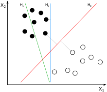
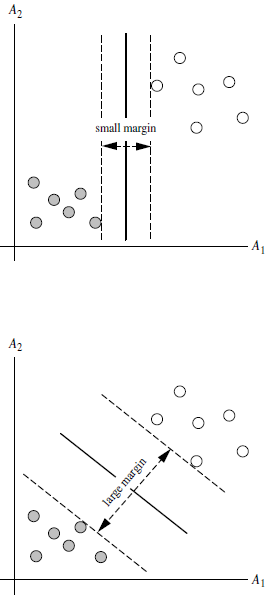
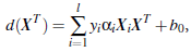
SVM 寻找区分两类的超平面(hyper plane), 使边际(margin)最大如何选取使边际(margin)最大的超平面 (Max Margin Hyperplane)？超平面到一侧最近点的距离等于到另一侧最近点的距离，两侧的两个超平面平行

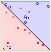
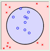
线性可区分(linear separable) 和线性不可区分 (linear inseparable)

4、定义与公式建立

超平面可以定义为：

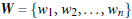
w: 权重向量，b: 偏置项 n：是特征值的个数 x: 特征向量

超平面方程为：

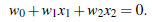
所有超平面右上方的点满足：

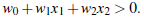
所有超平面左上方的点满足：

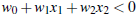
调整 weight，使超平面定义边际的两边：

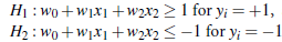
综合以上两式得到：

所有坐落在边际的两边的的超平面上的被称作”支持向量(support vectors)" 分界的超平面和 H1 或 H2 上任意一点的距离为 (i.e.: 其中||W||是向量的范数(norm))

所以最大边距距离为： 2/||W||

5、SVM 算法的优化目标

SVM 如何找出最大边际的超平面呢

利用一些的数学优化方法，比如拉格朗日乘子法，将上述的优化目标转化为一个凸二次规划问题，然后通过求解该凸二次规划问题，得到最优解，从而得到最大边际的超平面

对于任何测试（要归类的）实例，带入以上公式，得出的符号是正还是负决定

二、SVM 算法

1、SVM 算法示例

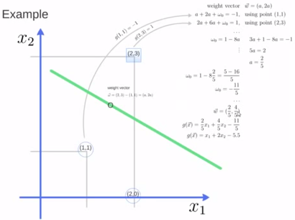
# SVM 是一种监督学习算法，常用于分类和回归任务
from sklearn import svm


x = [[2, 0], [1, 1], [2, 3]]
y = [0, 0, 1]
clf = svm.SVC(kernel = 'linear')
# fit 方法用于训练模型，它接收特征数据 x 和目标标签 y 作为输入。
clf.fit(x, y)

print(clf);

# get support vectors
print(clf.support_vectors_); # [[1. 1.] [2. 3.]]
# get indices of support vectors
print(clf.support_); # 打印支持向量的索引。
# get number of support vectors for each class
print(clf.n_support_); # 打印每个类别的支持向量数量。

使用 pridict 对新数据进行预测

from sklearn import svm
x = [[2, 0], [1, 1], [2, 3]]
y = [0, 0, 1]
clf = svm.SVC(kernel = 'linear')
clf.fit(x, y)
# 新数据点
new_data = [[1, 2], [3, 4]]

# 预测新数据点的类别
predictions = clf.predict(new_data)

print("Predictions:", predictions)

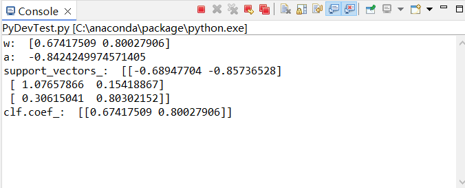
2、SVM 算法绘图

import numpy as np # 用于数值计算
import pylab as pl # 用于绘图
from sklearn import svm # 是 scikit-learn 中的支持向量机模块

# 创建两个类别的数据点，每个类别有 20 个样本。第一类数据点的均值为 [-2, -2]，第二类数据点的均值为 [+2, +2]。
X = np.r_[np.random.randn(20, 2) - [2, 2], np.random.randn(20, 2) + [2, 2]]
Y = [0]*20 +[1]*20

#fit the model
clf = svm.SVC(kernel='linear')
clf.fit(X, Y)

# 获取分离超平面
w = clf.coef_[0]
a = -w[0]/w[1]
xx = np.linspace(-5, 5)
yy = a*xx - (clf.intercept_[0])/w[1]

# 绘制支持向量和平行线
b = clf.support_vectors_[0]
yy_down = a*xx + (b[1] - a*b[0])
b = clf.support_vectors_[-1]
yy_up = a*xx + (b[1] - a*b[0])

print("w: ", w);
print("a: ", a);

# print("xx: ", xx);
# print("yy: ", yy);
print("support_vectors_: ", clf.support_vectors_);
print("clf.coef_: ", clf.coef_);

# switching to the generic n-dimensional parameterization of the hyperplan to the 2D-specific equation
# of a line y=a.x +b: the generic w_0x + w_1y +w_3=0 can be rewritten y = -(w_0/w_1) x + (w_3/w_1)


# 绘制图形
pl.plot(xx, yy, 'k-')
pl.plot(xx, yy_down, 'k--')
pl.plot(xx, yy_up, 'k--')

pl.scatter(clf.support_vectors_[:, 0], clf.support_vectors_[:, 1],
          s=80, facecolors='none')
pl.scatter(X[:, 0], X[:, 1], c=Y, cmap=pl.cm.Paired)

pl.axis('tight')
pl.show()

run 运行代码，得到如下结果：

3、人脸识别代码

from __future__ import print_function

from time import time
import logging
import matplotlib.pyplot as plt

from sklearn.model_selection import train_test_split  # 修改这里
from sklearn.datasets import fetch_lfw_people
from sklearn.model_selection import GridSearchCV      # 修改这里
from sklearn.metrics import classification_report
from sklearn.metrics import confusion_matrix
from sklearn.decomposition import PCA                # 修改这里
from sklearn.svm import SVC

print(__doc__)

# 显示日志
logging.basicConfig(level=logging.INFO, format='%(asctime)s %(message)s')

# 加载数据
lfw_people = fetch_lfw_people(min_faces_per_person=70, resize=0.4)
n_samples, h, w = lfw_people.images.shape
X = lfw_people.data
n_features = X.shape[1]
y = lfw_people.target
target_names = lfw_people.target_names
n_classes = target_names.shape[0]

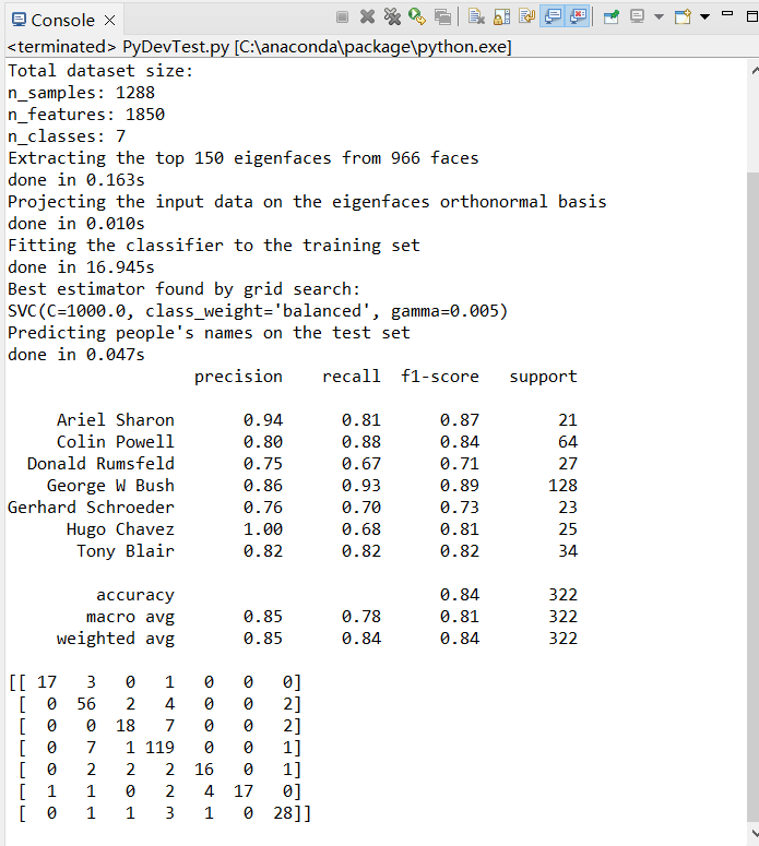
print("Total dataset size:")
print("n_samples: %d" % n_samples)
print("n_features: %d" % n_features)
print("n_classes: %d" % n_classes)

# 划分训练集和测试集
X_train, X_test, y_train, y_test = train_test_split(X, y, test_size=0.25)

# 使用PCA（主成分分析）
n_components = 150

print("Extracting the top %d eigenfaces from %d faces" % (n_components, X_train.shape[0]))
t0 = time()
# 将RandomizedPCA替换为PCA并设置svd_solver='randomized'
pca = PCA(n_components=n_components, whiten=True, svd_solver='randomized').fit(X_train)  # 修改这里
print("done in %0.3fs" % (time() - t0))

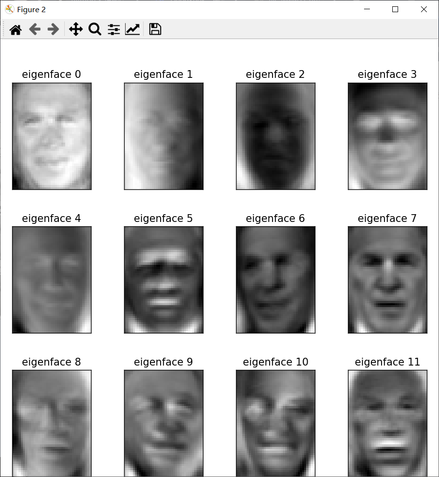
eigenfaces = pca.components_.reshape((n_components, h, w))

print("Projecting the input data on the eigenfaces orthonormal basis")
t0 = time()
X_train_pca = pca.transform(X_train)
X_test_pca = pca.transform(X_test)
print("done in %0.3fs" % (time() - t0))

# 训练SVM分类器
print("Fitting the classifier to the training set")
t0 = time()
param_grid = {'C': [1e3, 5e3, 1e4, 5e4, 1e5],
              'gamma': [0.0001, 0.0005, 0.001, 0.005, 0.01, 0.1]}
# 将class_weight='auto'改为'balanced'
clf = GridSearchCV(SVC(kernel='rbf', class_weight='balanced'), param_grid)  # 修改这里
clf = clf.fit(X_train_pca, y_train)
print("done in %0.3fs" % (time() - t0))
print("Best estimator found by grid search:")
print(clf.best_estimator_)

# 在测试集上评估模型
print("Predicting people's names on the test set")
t0 = time()
y_pred = clf.predict(X_test_pca)
print("done in %0.3fs" % (time() - t0))

print(classification_report(y_test, y_pred, target_names=target_names))
print(confusion_matrix(y_test, y_pred, labels=range(n_classes)))

# 可视化结果
def plot_gallery(images, titles, h, w, n_row=3, n_col=4):
    plt.figure(figsize=(1.8 * n_col, 2.4 * n_row))
    plt.subplots_adjust(bottom=0, left=.01, right=.99, top=.90, hspace=.35)
    for i in range(n_row * n_col):
        plt.subplot(n_row, n_col, i + 1)
        plt.imshow(images[i].reshape((h, w)), cmap=plt.cm.gray)
        plt.title(titles[i], size=12)
        plt.xticks(())
        plt.yticks(())

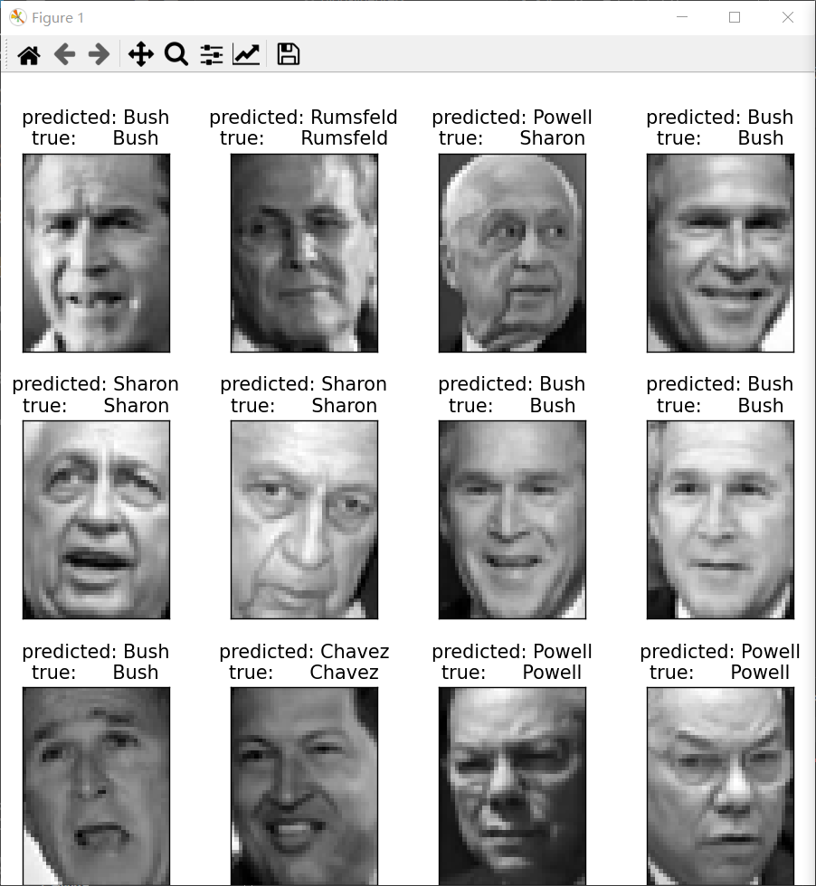
def title(y_pred, y_test, target_names, i):
    pred_name = target_names[y_pred[i]].rsplit(' ', 1)[-1]
    true_name = target_names[y_test[i]].rsplit(' ', 1)[-1]
    return 'predicted: %s\ntrue:      %s' % (pred_name, true_name)

prediction_titles = [title(y_pred, y_test, target_names, i) for i in range(y_pred.shape[0])]
plot_gallery(X_test, prediction_titles, h, w)

# 显示特征脸
eigenface_titles = ["eigenface %d" % i for i in range(eigenfaces.shape[0])]
plot_gallery(eigenfaces, eigenface_titles, h, w)

plt.show()

3.支持向量机SVM算法

目录